In this blog we will discuss one of the most imoprtant and powerful regularization techniques which is dropout, the focus of this blog won’t be on Implementing dropout, as it’s a straightforward implementation using common frameworks like Tensorflow, but we will instead focus on getting deeper intuition of what dropout is actually doing to the network and why it works at all with such a random nature.

Overview

The blog is divided into three sections:

• Introduction
• How it works?
• Intuitions

Introduction

Large networks are prone to overfitting, especially when they are trained on small datasets. With such networks, regularization is often essential, and one of the most used techniques for that is Dropout. In dropout units from network are dropped randomly during training based on a retention probability we specify for each layer, this simple technique helps reduce co-adaptation between units, and thus reduce overfitting.

Figure-1 from paper

How it works

One of the known regularization methods as well, is ensemble learning, in such a method you train different networks in parallel on often different datasets and then average their predictions at test time. Obviously, this technique requires a lot of computational resources in order to train many networks. Dropout addresses this problem, although it’s similar to ensemble learning in terms of involving many networks in training, the underneath process of training is totally different.

In dropout, random units are dropped in each training step (single iteration), resulting in a different smaller network (thinned network), the forward and backward propagatoins are implemented only on the resulting thinned network. As a result, when averaging the training steps of all thinned networks we end up with a single network that approximately represents all these thinned networks combined but with less computations and time needed.

think of it this way, each thinned network updates the weights once and then passes them to the next thinned network,a thinned network actually starts where the previous thinned network stopped, and weights keep updating in the same manner.

Figure-2

So thinned networks work in series rather than in parallel, they share the weights and participate in updating them sequentially. In dropout each layer is presented with a retention probability p, for instance, if a layer has a p value of 0.7, then roughly 30% (0.3) of units in that layer will be dropped randomly along with their incoming and outgoing connections. At test time no units are dropped and the whole network is utilized to make predictions. Therefore When dropout is eliminated, units receive more connections from the previous layer than what they used to during training and thus become overexcited. To overcome the effect of overexcitation all weights in a layer are multiplied by the retention probability associated with that layer. We eventually end up with an unthinned network that has smaller weights and approximately represents the effect of averaging the predictions of all these thinned networks.

Figure-3 from paper

Intuitions:

In this section we will discuss the following:

1. The effect of retention probability and why it’s recommended to be set closer to 0.5 or higher not lower?
2. How this reduces overfitting?

The effect of retention probability and why it’s recommended to be set closer to 0.5 or higher not lower?

Imagine setting the value of p to be very small (p=0.01) for all hidden layers, and for the sake of this example assume the network to have only one hidden layer of 100 units, as a result, the produced thinned networks will almost be of 1 unit, which are 100 times smaller than the original network. This will destroy the network and completely wipe out the co-adaptation that could exist between units as each unit is trained individually in that case, in other words, this will cause complete randomness and the network won’t propagate any useful information. The goal then isn’t to completely wipe out co-adaptation, but to (reduce) it, by causing some randomness to the network that lets generalization takes place and hopefully reduce overfitting. In the same network above, when using p value of 0.5 or higher instead, the thinned networks will be at most 2 times smaller if not less, this will allow units to work together (adapt to some extent and capture useful patterns) and train in an environment that is similar to that used at inference time.

This as well explains why the network works so well at inference time when randomness is suddenly eliminated, as when using p values larger than 0.5 we are not causing a high degree of randomness, that’s in addition to multiplying weights by p after training to prevent overexcitation. All these play roles in making the network performs well at test time.

How this reduces overfitting?

As discussed above, in dropout each unit is trained in many different networks, which in return reduces co-adaptation between units, this has the effect of forcing units to be as useful as possible on their own.

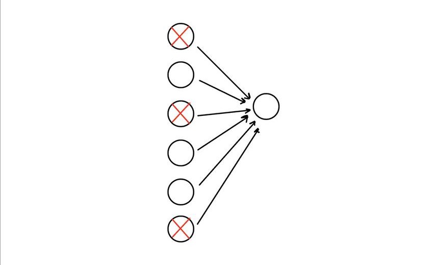Figure-4

As in the above image when implementing dropout, the next-layer unit can’t rely heavily on just one of the inputs, it has to pay attention to all of them, which means spreading out the weight rather than putting to much weight on a single input (this has similar effect of shrinking weights as in L2 regularization method). Units then become less sensitive to slight changes in the inputs and therefore makes the network generalizes much better.